Draw A Rectangle - Demo 02
Objective
Learn how to draw rectangles in an OpenGL window. Learn about OpenGL’s coordinate system, Normalized Device Coordinates (NDC), which are from -1.0 to 1.0, in the X, Y, and Z directions. Geometry drawn outside of this region will not be displayed in the window.
Demo 02
How to Execute
Load src/modelviewprojection/demo02.py in Spyder and hit the play button.
Code
GLFW/OpenGL Initialization
The setup code is the same. Initialize GLFW. Set the OpenGL version. Create the window. Set a key handler for closing. Set the background to be black. Execute the event/drawing loop.
The Event Loop
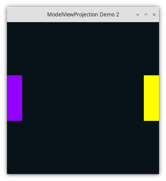
Within the event loop, demo02.py draws 2 rectangles, as one might see in a game of Pong.
52while not glfw.window_should_close(window):
...
Draw Paddles
The black screen from demo01 is not particularly interesting, so let’s draw something, say, two rectangles. To do this, we need to figure out what colors to use, and the positions of the rectangles in NDC. “glColor3f” is a function sets a global variable, which makes it the color to be used for the subsequently-drawn graphical shape(s). Lets make the first paddle purple, and a second paddle yellow.
To specify the corners of the rectangle, “glBegin(GL_QUADS)” tells OpenGL that we will soon specify 4 vertices, (i.e. points) which define the quadrilateral. The vertices will be specified by calling “glVertex2f” 4 times.
Calling the “glEnd()” function tells OpenGL that we have finished providing vertices for the quadrilateral.
Draw Paddle 1
61    GL.glColor3f(0.578123, 0.0, 1.0)
62    GL.glBegin(GL.GL_QUADS)
63    GL.glVertex2f(-1.0, -0.3)  # vertex C
64    GL.glVertex2f(-0.8, -0.3)  # vertex D
65    GL.glVertex2f(-0.8, 0.3)  # vertex A
66    GL.glVertex2f(-1.0, 0.3)  # vertex B
67    GL.glEnd()
The paddle looks like this relative to NDC:

Rectangle
Draw Paddle 2
71    GL.glColor3f(1.0, 1.0, 0.0)
72    GL.glBegin(GL.GL_QUADS)
73    GL.glVertex2f(0.8, -0.3)  # vertex G
74    GL.glVertex2f(1.0, -0.3)  # vertex H
75    GL.glVertex2f(1.0, 0.3)  # vertex E
76    GL.glVertex2f(0.8, 0.3)  # vertex F
77    GL.glEnd()
The 2 paddles looks like this relative to NDC:

Rectangle
81 glfw.swap_buffers(window)
done with frame, flush the current buffer to the monitor
Swap front and back buffers
The frame sent to the monitor is a set of values like this
bbbbbbbbbbbbbbbbbbbbbbbbbbbbbbbbbbbbb
bbbbbbbbbbbbbbbbbbbbbbbbbbbbbbbbbbbbb
bbbbbbbbbbbbbbbbbbbbbbbbbbbbbbbbbbbbb
PPPPPbbbbbbbbbbbbbbbbbbbbbbbbbbbRRRRR
PPPPPbbbbbbbbbbbbbbbbbbbbbbbbbbbRRRRR
PPPPPbbbbbbbbbbbbbbbbbbbbbbbbbbbRRRRR
PPPPPbbbbbbbbbbbbbbbbbbbbbbbbbbbRRRRR
PPPPPbbbbbbbbbbbbbbbbbbbbbbbbbbbRRRRR
PPPPPbbbbbbbbbbbbbbbbbbbbbbbbbbbbbbbb
bbbbbbbbbbbbbbbbbbbbbbbbbbbbbbbbbbbbb
bbbbbbbbbbbbbbbbbbbbbbbbbbbbbbbbbbbbb
bbbbbbbbbbbbbbbbbbbbbbbbbbbbbbbbbbbbb
What do we have to do to convert from NDC (i.e. (1.0, 0.8)) into pixel coordinates (i.e. pixel (10,15))? Nothing, OpenGL does that for us automatically; therefore we never have to think in terms of pixels coordinates, only in terms of vertices of shapes, specified using coordinates relative to NDC. OpenGL also automatically colors all of the pixels which are inside of the quadrilateral.
Why do we use NDC instead of pixel coordinates?
Normalized-Device-Coordinates
The author owns two monitors, one which has 1024x768 pixels, and one which has 1920x1200 pixels. When he purchases a video game, he expects that his game will run correctly on either monitor, in full-screen mode. If a graphics programmer had to explicitly set the color of individual pixels using the pixel’s coordinates, the the programmer would have to program using “screen-space” (Any space means a system of numbers which you’re using. Screen-space means you’re specifically using pixel coordinates, i.e, set pixel (5,10) to be yellow).
What looks alright in screen-space on a large monitor…

Screenspace
Isn’t the same picture on a smaller monitor.

Screenspace
Like any good program or library, OpenGL creates an abstraction. In this case, it abstracts over Screen Space, thus freeing the programmer from caring about screen size. Since a programmer does not want to program in discrete (discrete means integer values, not continuous) screen-space, what type of numbers should he use? Firstly, it should be a continuous space, because if a real-world object is 10.3 meters long, a programmer should be able to enter “float foo = 10.3”. Secondly, it should be a fixed range vertically and an fixed range horizontally. OpenGL will have to convert points from some space to screen-space, and since this is done in hardware (i.e. you can’t pragmatically change how the conversion happens), it should be a fixed size.
OpenGL uses what’s called :term:`NDC<Normalized Device Coordinates>`, which is a continuous space from -1.0 to 1.0 horizontally, -1.0 to 1.0 vertically, and from -1.0 to 1.0 depth-ally. (Is there an actual word for that???)

NDC space
It should look the same whether we own a small monitor (ignoring aspect ratio, for now).

NDC space
Or a large monitor.
NDC space
Introduction to Cayley Graphs
The following is a graph [Tru93], specifically a Cayley Graph [1] [Pin90], of the two spaces shown so far. The nodes represent a coordinate system (i.e. origin and axes), and the directed edge represents an invertible function that converts coordinates from one coordinate system to another. If this isn’t clear to the reader, look above at the 3 pictures of the 2 quadrilaterals. They look the same, but if you label each vector on all three graphs, and look at the axes to find their plotted values, you will find that they differ. Changing between coordinate systems means to take vertices from one coordinate system and changing them to another, like converting from Celsius to Fahrenheit, meters to feet, etc.
NDC/Screenspace Conversion
Demo 02
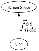
The function that converts from Normalized Device Coordinates to Screen Space is arbitrarily named “f”, sub-scripted by “ndc”, super-scripted by “ss”. This is a notation for naming functions that change basis, i.e. coordinate conversion. A definition of this function is not provided right now, because we can’t change it in software, but we must recognize that it exists.
The Wikipedia article for Cayley graphs (https://en.wikipedia.org/wiki/Cayley_graph) is intimidating, but for our purposes, the use of Cayley graphs is very simple.
Currency Conversion
An univariate example use of Cayley graphs is exchanging coins with a bank.
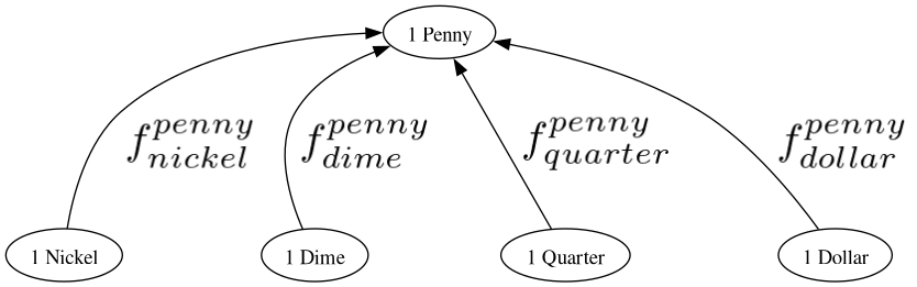
Cayley graph of univariate coordinate conversion for money.
The directed edges in the Cayley graph show the direction that the function, i.e. transformation, applies.
To convert 20 nickels into pennies, start at nickel, move to penny, while applying the appropriate function along the way.
To convert those 100 pennies into quarters, on the Cayley graph, move from penny to quarter, but since we are moving in the opposite direction of the edge, we must apply the multiplicative inverse of that function. These functions are invertible by taking the reciprocal of the coefficient
By taking the inverse of the coefficient, we satisfy a definition of an inverse
To convert between any denomination, say dimes to dollars, just compose the functions, remembering to take the inverse of any directed edge that you against.
Notice in the last equation that we defined the function via function composition, and didn’t specify any arguments. We just focus on the types of units in and the units out, but the details of those functions are not relevant when traversing the Cayley graph.
Function composition is used extensively throughout this book. As a reminder
Given that the compose operation is on the functions, another way of writing it omits the argument \(x\)
Temperature Conversion
Another univariate example use of Cayley graphs is converting a temperature between different units of measure.

Cayley graph of univariate coordinate conversion for temperature.
Given that those functions are invertible, with the Cayley graph and the function definitions, we have the information needed to convert a temperature values any other unit of temperature. When creating the graph, we don’t think about how to do every pair of conversions, because they can be created later by using function composition, and/or taking the inverse of given functions.
To convert from fahrenheit to kelvin
To convert from kelvin to celsius
To convert from celsius to fahrenheit
To convert from kelvin to fahrenheit
Learning what to ignore
A big part of being able to understand graphics well is being able to figure out what to ignore. To quote Gerald Sussman in the SICP video lectures “”One of the things that we have to learn how to do, is to ignore details. The key to understanding complicated things is to know what not to look, and what not to compute, and what not to think.”
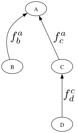
Below is a Cayley graph that shows coordinate systems “a”, “b”, “c”, and “d”, and functions are provided to us to convert between some of the spaces. What do those names “a”, “b”, “c”, and “d” mean? It doesn’t matter. What is the definition of all of the functions? It doesn’t matter. All that matters
is that the function exists
the function is invertible
Generic Cayley Graph
So how would we convert coordinates from space D to space B? We know that D is defined relative to C, C is defined relative to A, and B is defined relative to A. Because of the arrows, we know that we are given a definition for a function from D to C, for a function from C to A, and for a function from B to A. We are not directly given their inverses, but we can calculate them easily enough, or have a computer do it for us.
In tracing out the graph, we are going with the first two directed edges, and against the last one. So we compose the functions and take the appropriate inverse(s).
A function from A to B is not provided to us, but we wrote it in the equation as an idea of a function that we wish to have, even though we don’t currently have it. However, we can create this function by invoking inverse on the provided function from A to B.
Since we’re dealing with function composition, we don’t even need to specify the argument
If this seems to abstract for now, don’t worry. By the end of the course, it should be clear. The goal of this book is to make it clear, and then, obvious.
Exercise
Run Demo 2. Resize the window using the GUI controls provided by the Operating system. first make it skinny, and then wide. Observe at what happens to the rectangles.