Modelspace - Demo 06¶

Objective¶

Learn about modelspace Modelspace.

How to Execute¶

Load src/modelviewprojection/demo06.py in Spyder and hit the play button.

Move the Paddles using the Keyboard¶

Keyboard Input	Action
w	Move Left Paddle Up
s	Move Left Paddle Down
k	Move Right Paddle Down
i	Move Right Paddle Up

Modelspace¶

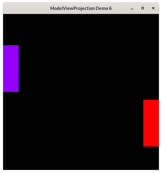
NDC are not a natural system of numbers for use by humans. Imagine that the paddles in the previous chapters exist in real life, and are 2 meters wide and 6 meters tall. The graphics programmer should be able to use those numbers directly; they shouldn’t have to manually transform the distances into NDC.

Whatever a convenient numbering system is (i.e. coordinate system) for modeling objects is called modelspace. Since a paddle has four corners, which corner should be at the origin (0,0)? If you don’t already know what you want at the origin, then none of the corners should be; instead put the center of the object at the origin (Because by putting the center of the object at the origin, scaling and rotating the object are trivial, as shown in later chapters).

modelspace - the coordinate system (origin plus axes), in which some object’s vertices are defined.

WorldSpace¶

WorldSpace is a top-level space, independent of NDC, that we choose to use. It is arbitrary. If you were to model a racetrack for a racing game, the origin of WorldSpace may be the center of that racetrack. If you were modeling our solar system, the center of the sun could be the origin of “WorldSpace”. I personally would put the center of our flat earth at the origin, but reasonable people can disagree.

For our demo with paddles, the author arbitrarily defines the WorldSpace to be 20 units wide, 20 units tall, with the origin at the center.

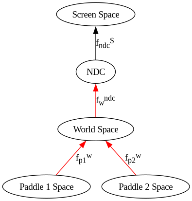
Modelspace to WorldSpace¶

The author prefers to view transformations as changes to the graph paper, as compared to view transformations as changes to points.

As such, for placing paddle1, we can view the translation as a change to the graph paper relative to world space coordinates (only incidentally bringing the vertices along with it) and then resetting the graph paper (i.e. both origin and axes) back to its original position and orientation. Although we will think of the paddle’s vertices as relative to its own space (i.e. -1 to 1 horizontally, -3 to 3 vertically), we will not look at the numbers of what they are in world space coordinates, as doing so

Will not give us any insight
Will distract us from thinking clearly about what’s happening
As an example, figure out the world space coordinate of the upper rights corner of the paddle after it has been translated, and ask yourself what that means and what insight did you gain?

The animation above shows multiple steps, shown now without animation.

Modelspace of Paddle 1¶

Paddle 1's Modelspace — Paddle 1’s Modelspace¶

Vector	Coordinates
a	(1,3)
b	(-1,3)
c	(-1,-3)
d	(1,-3)

Modelspace of Paddle 1 Superimposed on Worldspace after the translation¶

Paddle 1’s graph paper gets translated -9 units in the x direction, and some number of units in the y direction, 0 during the first frame, based off of user input. The origin is translated, and the graph paper comes with it, onto which you can plot the vertices. Notice that the coordinate system labels below the plot and to the left of the plot is unchanged. That is world space, which has not changed.

Paddle 1's Modelspace Superimposed on World Space — Paddle 1’s Modelspace Superimposed on World Space¶

Vector	Coordinates (modelspace)	Coordinates (worldspace)
a	(1,3)	(1,3) + (9,3) = (-8,5)
b	(-1,3)	(-1,3) + (9,3) = (-10,5)
c	(-1,-3)	(-1,-3) + (9,3) = (-10,-1)
d	(1,-3)	(1,-3) + (9,3) = (-8,-1)

Paddle 1’s vertices in WorldSpace Coordinates¶

Vector	Coordinates (worldspace)
a	(-8,5)
b	(-10,5)
c	(-10,-1)
d	(-8,-1)

Now that the transformation has happened, the vertices are all in world space. You could calculate their values in world space, but that will not give you any insight. The only numbers that matter for insight as that the entire graph paper of modelspace, which originally was the same as world space, has changed, bringing the vertices along with it.

Same goes for Paddle 2’s modelspace, relative to its translation, which are different values.

Modelspace of Paddle 2¶

Vector	Coordinates
a	(1,3)
b	(-1,3)
c	(-1,-3)
d	(1,-3)

Modelspace of Paddle 2 Superimposed on Worldspace after the translation¶

Vector	Coordinates (modelspace)	Coordinates (worldspace)
a	(1,3)	(1,3) + (9,-4) = (10,-1)
b	(-1,3)	(-1,3) + (9,-4) = (8,-1)
c	(-1,-3)	(-1,-3) + (9,-4) = (8,-7)
d	(1,-3)	(1,-3) + (9,-4) = (10,-7)

Paddle 2’s vertices in WorldSpace Coordinates¶

Vector	Coordinates (worldspace)
a	(10,-1)
b	(8,-1)
c	(8,-7)
d	(10,-7)

Scaling¶

Our paddles are now well outside of NDC, and as such, they would not be displayed, as they would be clipped out. Their values are outside of -1.0 to 1.0. All we will need to do to convert them from world space to NDC is divide each component, x and y, by 10.

As a demonstration of how scaling works, let’s make an object’s width twice as large, and height three times as large. (The author tried doing the actual scaling of 1/10 in an animated gif, and it looked awful, therefore a different scaling gif is showed here, but the concept is the same).

We can expand or shrink the size of an object by “scale”ing each component of the vertices by some coefficient.

Worldspace. Don’t concern yourself with what the numbers are.¶

Our global space is -10 to 10 in both dimensions, and to get it into NDC, we need to scale by dividing by 10

\[\begin{split}\begin{bmatrix} x_{w} \\ y_{w} \end{bmatrix} = \vec{f}_{p1}^{w}( \begin{bmatrix} x_{p1} \\ y_{p1} \end{bmatrix}) = \begin{bmatrix} x_{p1} \\ y_{p1} \end{bmatrix} + \begin{bmatrix} {p1}_{x} \\ {p1}_{y} \end{bmatrix}\end{split}\]

where x_p1, y_p1 are the modelspace coordinates of the paddle’s vertices, and where p1_center_x_worldspace, p1_center_y_worldspace, are the offset from the world space’s origin to the center of the paddle, i.e. the translation.

\[\begin{split}\begin{bmatrix} x_{w} \\ y_{w} \end{bmatrix} = \vec{f}_{p2}^{w} ( \begin{bmatrix} x_{p2} \\ y_{p2} \end{bmatrix}) = \begin{bmatrix} x_{p2} \\ y_{p2} \end{bmatrix} + \begin{bmatrix} {p2}_{x} \\ {p2}_{y} \end{bmatrix}\end{split}\]

Now, the coordinates for paddle 1 and for paddle 2 are in world space, and we need the match to take any world space coordinates and convert them to NDC.

\[\begin{split}\begin{bmatrix} x_{ndc} \\ y_{ndc} \end{bmatrix} = \vec{f}_{w}^{ndc} ( \begin{bmatrix} x_{w} \\ y_{w} \end{bmatrix}) = 1/10 * \begin{bmatrix} x_{w} \\ y_{w} \end{bmatrix}\end{split}\]

Modelviewprojection comes with a math library, the 2D version is named “mathutils2d.py”. The main class in this module is “Vector2D”, which has two components: and x value, and a y value. To add a vector2d to another one on the right hand side of the ‘+’ symbol, we just add the respective components together, and create a new Vector2D.

src/modelviewprojection/mathutils2d.py¶

@dataclass
class Vector2D:
    x: float  #: The x-component of the 2D Vector
    y: float  #: The y-component of the 2D Vector

In a Python class, we can overload the ‘+’ symbol, to make objects addable, by implementing the ‘__add__’ method.

src/modelviewprojection/mathutils2d.py¶

    def __add__(self, rhs: Vector2D) -> Vector2D:
        """
        Add together two Vector2Ds.

        Let :math:`\\vec{a} = \\begin{pmatrix} a_x \\\\ a_y \\end{pmatrix}`
        and :math:`\\vec{b} = \\begin{pmatrix} b_x \\\\ b_y \\end{pmatrix}`:

        .. math::

             \\vec{a} + \\vec{b} = \\begin{pmatrix} a_x + b_x \\\\ a_y + b_y \\end{pmatrix}

        Args:
            rhs (Vector2D): The vector on the right hand side of the addition
                            symbol
        Returns:
            Vector2D: The Vector2D that represents the additon of the two
                      input Vector2Ds
        Raises:
            Nothing
        Example:
            >>> from modelviewprojection.mathutils2d import Vector2D
            >>> a = Vector2D(x=2.0, y=3.0)
            >>> b = Vector2D(x=5.0, y=6.0)
            >>> a + b
            Vector2D(x=7.0, y=9.0)
        """

        return Vector2D(x=(self.x + rhs.x), y=(self.y + rhs.y))

We can also model the opposite procedure, subtraction, by implementing the “__sub__” method.

src/modelviewprojection/mathutils2d.py¶

    def __sub__(self, rhs: Vector2D) -> Vector2D:
        """
        Subtract the right hand side Vector2D from the left hand side Vector2D.

        Let :math:`\\vec{a} = \\begin{pmatrix} a_x \\\\ a_y \\end{pmatrix}`
        and :math:`\\vec{b} = \\begin{pmatrix} b_x \\\\ b_y \\end{pmatrix}`:

        .. math::

             \\vec{a} - \\vec{b} = \\vec{a} + \\vec{b} = \\begin{pmatrix} a_x - b_x \\\\ a_y - b_y \\end{pmatrix}

        Args:
            rhs (Vector2D): The vector on the right hand side of the
                            subtraction symbol
        Returns:
            Vector2D: The Vector2D that represents the subtraction of the
                      right hand side Vector2D from the left hand side
                      Vector2D
        Raises:
            Nothing
        Example:
            >>> from modelviewprojection.mathutils2d import Vector2D
            >>> a = Vector2D(x=2.0, y=3.0)
            >>> b = Vector2D(x=5.0, y=2.0)
            >>> a - b
            Vector2D(x=-3.0, y=1.0)
        """
        return Vector2D(x=(self.x - rhs.x), y=(self.y - rhs.y))

In our graphics code, instead of using “a+b”, we’ll use a more descriptive name: “translate”, which is implemented using the addition symbol. But a few things to note, “translate” is a function on the mathutils module, not a method on Vector2D class, and it’s wrapped in a class named “InvertibleFunction”

src/modelviewprojection/mathutils2d.py¶

def translate(b: Vector2D) -> InvertibleFunction[Vector2D]:
    def f(vector: Vector2D) -> Vector2D:
        return vector + b

    def f_inv(vector: Vector2D) -> Vector2D:
        return vector - b

    return InvertibleFunction[Vector2D](f, f_inv)

Notice in particular that the “b” parameter is passed as an argument to “translate”, but the function for translating, named “f”, and the inverse of “f” named “f_inv”, take a Vector2D. This is because we will be translating many Vector2Ds using the same amount.

Invertible functions are stored in pairs, with the “active” function being the first one passed to the constructor. So for translate above, the adding of the Vector2Ds will be the function, but InvertibleFunction holds onto the second function, for later use to be able to undo the function’s application.

tests/test_mathutils2d.py¶

def test_translate():
    fn: InvertibleFunction[Vector2D] = translate(Vector2D(x=2.0, y=3.0))
    fn_inv: InvertibleFunction[Vector2D] = inverse(fn)

    input_output_pairs = [
        [[0.0, 0.0], [2.0, 3.0]],
        [[1.0, 0.0], [3.0, 3.0]],
        [[0.0, 1.0], [2.0, 4.0]],
    ]

    for input_val, output_val in input_output_pairs:
        wrap_vec2_test(fn, input_val, output_val)
        wrap_vec2_test(fn_inv, output_val, input_val)

The above is a unit test that shows how the translate function can be used. We call “translate”, a function which takes a translate amount, both in the x direction and the y direction, but we have not yet specified what needs to be translated by that amount. “translate” returns an InvertibleFunction, which is Callable[Vector2D, Vector2D]. Callable[Vector2D, Vector2D] is a type which is a function that takes a Vector2D as input, and returns a Vector2D (in this case, the output is the input, translated by Vector2D(x=2.0, y=3.0).

On the next 3 lines, we call the function t, passing in a Vector2D to be translated, and we test if the result is equal to the specified amount. (“approx”, is a function from the pytest module, which when tested for equality, returns true if the two floating point numbers under comparison are “close enough”).

We then define a function t_inv, by calling “inverse” on function “t”. We then see that composing t_inv and t results in no transformation.

Here’s how InvertibleFunction is implemented:

src/modelviewprojection/mathutils.py¶

# Define a generic type variable
T = TypeVar("T")


@dataclass
class InvertibleFunction(Generic[T]):
    """
    Class that wraps a function and its
    inverse function.  The function takes
    type T as it's argument and it's evaluation
    results in a value of type T.
    """

    func: Callable[[T], T]  #: The wrapped function
    inverse: Callable[[T], T]  #: The inverse of the wrapped function

    def __call__(self, x: T) -> T:
        """
        Execute a function with the given value.

        Args:
            func (Callable[[T], T]): A function that takes a value of type T
                                     and returns a value of the same type T.
            value (T): The input value to pass to the function
        Returns:
            T: The result of calling func(value). Will be the same type as the
                input value.
        Raises:
            Nothing
        Example:
            >>> from modelviewprojection.mathutils import InvertibleFunction
            >>> from modelviewprojection.mathutils import inverse
            >>> def f(x):
            ...     return 2 + x
            ...
            >>> def f_inv(x):
            ...     return x - 2
            ...
            >>> foo = InvertibleFunction(func=f, inverse=f_inv)
            >>> foo # doctest: +ELLIPSIS
            InvertibleFunction(func=<function f at 0x...>, inverse=<function f_inv at 0x...>)
            >>> foo(5)
            7
            >>> inverse(foo) # doctest: +ELLIPSIS
            InvertibleFunction(func=<function f_inv at 0x...>, inverse=<function f at 0x...>)
            >>> inverse(foo)(foo(5))
            5
        """
        return self.func(x)


def inverse(f: InvertibleFunction[T]) -> InvertibleFunction[T]:
    """
    Get the inverse of the InvertibleFunction

    Args:
        f: InvertibleFunction[T]: A function with it's associated inverse
           function.
    Returns:
        InvertibleFunction[T]: The Inverse of the function
           function.
    Raises:
        Nothing
    Example:
        >>> from modelviewprojection.mathutils import InvertibleFunction
        >>> from modelviewprojection.mathutils import inverse
        >>> def f(x):
        ...     return 2 + x
        ...
        >>> def f_inv(x):
        ...     return x - 2
        ...
        >>> foo = InvertibleFunction(func=f, inverse=f_inv)
        >>> foo # doctest: +ELLIPSIS
        InvertibleFunction(func=<function f at 0x...>, inverse=<function f_inv at 0x...>)
        >>> foo(5)
        7
        >>> inverse(foo) # doctest: +ELLIPSIS
        InvertibleFunction(func=<function f_inv at 0x...>, inverse=<function f at 0x...>)
        >>> inverse(foo)(foo(5))
        5
    """

    return InvertibleFunction(f.inverse, f.func)

Just as Python allows an object to override the ‘+’ and ‘-’ syntax, in Python, any object can be treated as a function, by implementing the “__call__” method

Back to method’s on the Vector2D class. We can also define scaling of a Vector2D, by implementing multiplication of Vector2D’s by a scalar, meaning a real number that scaled the Vector2D by the same amount in all directions. We do this by implementing the ‘__mul__’ and ‘__rmul__’ methods, where __rmul__ just means that this object is on the right hand side of the multiplication.

src/modelviewprojection/mathutils2d.py¶

    def __mul__(self, scalar: float) -> Vector2D:
        """
        Multiply the Vector2D by a scalar number

        Let :math:`\\vec{a} = \\begin{pmatrix} a_x \\\\ a_y \\end{pmatrix}` and constant scalar :math:`s`:

        .. math::

             s*\\vec{a} = \\begin{pmatrix} s*a_x \\\\ s*a_y \\end{pmatrix}

        Args:
            rhs (Vector2D): The scalar to be multiplied to the Vector's component
                            subtraction symbol
        Returns:
            Vector2D: The Vector2D that represents scalar times the amount of the input Vector2D

        Raises:
            Nothing
        Example:
            >>> from modelviewprojection.mathutils2d import Vector2D
            >>> a = Vector2D(x=2.0, y=3.0)
            >>> a * 4
            Vector2D(x=8.0, y=12.0)
        """
        return Vector2D(x=(self.x * scalar), y=(self.y * scalar))

    def __rmul__(self, scalar: float) -> Vector2D:
        return self * scalar

Just like we made a top level invertible function called “translate” for addition, we are going to do the same for multiplication, and call it “uniform_scale”. Notice in particular that the scalar is passed as an argument to “uniform_scale”, but the function for scaling “f”, and the inverse of “f” named “f_inv”, take a Vector2D. This is because we will be scaling many Vector2Ds using the same scaling factor.

src/modelviewprojection/mathutils2d.py¶

def uniform_scale(m: float) -> InvertibleFunction[Vector2D]:
    def f(vector: Vector2D) -> Vector2D:
        return vector * m

    def f_inv(vector: Vector2D) -> Vector2D:
        if m == 0.0:
            raise ValueError("Note invertible.  Scaling factor cannot be zero.")

        return vector * (1.0 / m)

    return InvertibleFunction[Vector2D](f, f_inv)

NEW – Add the ability to scale a vector, to stretch or to shrink